Nonlinear Problems in One Variable

What Is Not Possible

Solvers can only return an approximate answer or signal that no solution was found in the allotted time.

Exercise 1

def Newtons_Method(f, f_prime, x_c):
    return x_c - f(x_c) / f_prime(x_c)

f = lambda x: x**4 - 12 * x**3 + 47 * x**2 - 60 * x
f_prime = lambda x: 4 * x**3 - 36 * x**2 + 94 * x - 60

x_c = 2
for i in range(5):
    x = Newtons_Method(f, f_prime, x_c)
    print('Iteration {0}: {1}'.format(i, x))
    x_c = x

Iteration 0: 2.75
Iteration 1: 2.954884105960265
Iteration 2: 2.997853245312536
Iteration 3: 2.99999465016014
Iteration 4: 2.9999999999666165

x_c = 1
for i in range(12):
    x = Newtons_Method(f, f_prime, x_c)
    print('Iteration {0}: {1}'.format(i, x))
    x_c = x

Iteration 0: 13.0
Iteration 1: 10.578892912571133
Iteration 2: 8.78588342536825
Iteration 3: 7.469644320482534
Iteration 4: 6.517931578972248
Iteration 5: 5.848418791850394
Iteration 6: 5.4023336439265215
Iteration 7: 5.139173220737766
Iteration 8: 5.024562327545462
Iteration 9: 5.000967258633622
Iteration 10: 5.000001586728139
Iteration 11: 5.000000000004287

Exercise 2

On CDC machines, the base is 2 and the mantissa has 48 bits. The machine is accurate up to \(\log 2^{48} \sim \log 10^{14.4} \approx 14\) decimal digits.

Given \(x_k = 1 + 0.9^k\), \(x_k \rightarrow 1\) implies

\[\begin{split}2^{-48} &= 0.9^k\\ -48 \log{2} &= k \log{0.9}\\ \frac{-48 \log{2}}{\log{0.9}} &= k \sim 315.78\end{split}\]

Evidently, it will take \(\lceil k \rceil\) iterations to converge to \(1\) on a CDC machine. The convergence rate is given by

\[\begin{split}\lvert x_{k + 1} - x_* \rvert &\leq c \lvert x_k - x_* \rvert\\ \left| \frac{0.9^{k + 1}}{0.9^{k}} \right| &\leq c\\ 0.9 \leq c,\end{split}\]

which shows that \(q\)-linear convergence with constant 0.9 is not satisfactory for general computational algorithms.

Exercise 3

The sequence \(x_k = 1 + 1 / k!\) converges \(q\)-superlinearly to one because

\[\begin{split}\left| \frac{\frac{1}{(k + 1)!}}{\frac{1}{k!}} \right| &\leq c\\ \left| \frac{1}{k + 1} \right| &\leq c.\end{split}\]

import matplotlib.pyplot as plt
import numpy

f = lambda x: 1 + 1 / numpy.math.factorial(x)
x_star = 1

C = []
for i in range(1, 20):
    x_k = f(i - 1)
    x_kp1 = f(i)

    C.append(abs(x_kp1 - x_star) / abs(x_k - x_star))
plt.plot(C)
plt.xlabel(r'Iteration $k$')
plt.ylabel('Convergence Rate')
plt.title(r'$1 + 1 / k! \rightarrow 1$')
plt.show()

<Figure size 640x480 with 1 Axes>

Exercise 4

See [Pot89] for details.

Exercise 5

Given \(\left\{ x_k \right\}\) has \(q\)-order at least \(p\) and \(e_k = |x_k - x_*|\), let \(b_k = |x_{k - 1} - x_*|\). By definition of \(q\)-order at least \(p\), \(\left\{ b_k \right\}\) converges to zero where \(e_k \leq b_k\) and \(\left| x_k - x_* \right| \leq c \left| x_{k - 1} - x_* \right|^p\) holds.

Applying L’Hopital’s rule to the following indeterminate form

\[\lim_{k \to \infty} \frac{b_k}{e_k} = \lim_{k \to \infty} \frac{\left| x_{k - 1} - x_* \right|}{\left| x_k - x_* \right|} = 1 < \infty\]

demonstrates convergence to a finite value.

Exercise 6

See [Gay79] for details.

Exercise 7

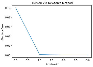
To reuse the framework of Newton’s method covered so far, we need to formulate a local model around \(f(x) = 1 / a\) such that we can solve for the root of the model.

Defining \(f(x) = a x - 1\) is perfectly valid and does not use any division operators. Unfortunately, this model still requires a division by \(f\) and \(f'\) for Newton’s method. To avoid those divisions, the model should be written as \(f(x) = 1 / x - a\) with \(f'(x) = -1 / x^2\).

\[\begin{split}f(x) - f(x_c) &= \int_{x_c}^x f'(z) dz\\ f(x) - f(x_c) &\simeq f'(x_c) (x - x_c) & \quad & \text{Taylor expansion}\\ x &= x_c + \frac{f(x) - f(x_c)}{f'(x_c)}\\ x_* &= x_c - \frac{f(x_c)}{f'(x_c)}\\ x_* &= x_c - \frac{1 / x_c - a}{-1 / x_c^2}\\ x_* &= x_c + x_c - a x_c^2\\ x_* &= x_c (2 - a x_c)\end{split}\]

The absolute error

\[\begin{split}\left| x_k - x_* \right| &\leq \left| x_{k - 1} (2 - a x_{k - 1}) - \frac{1}{a} \right|\\ &\leq \left| -a x_{k - 1}^2 + 2 x_{k - 1} - \frac{1}{a} \right|\\ &\leq \left| a x_{k - 1}^2 - 2 x_{k - 1} + \frac{1}{a} \right|\\ &\leq |a| \left| x_{k - 1}^2 - \frac{2}{a} x_{k - 1} + \frac{1}{a^2} \right|\\ &\leq |a| \left| x_{k - 1} - \frac{1}{a} \right|^2\end{split}\]

indicates the convergence rate is \(q\)-quadratic.

import matplotlib.pyplot as plt

a = 9
f = lambda x_c: x_c * (2 - a * x_c)
x_star = 1 / a
x_c = round(1 / a, 1)
C = [x_c]
for i in range(3):
    x_k = f(x_c)
    x_c = x_k

    C.append(abs(x_k - x_star))
plt.plot(C)
plt.xlabel(r'Iteration $k$')
plt.ylabel('Absolute Error')
plt.title("Division via Newton's Method")
plt.show()

Exercise 8

Define \(D = \left| x_0 - z_0 \right|\) as the length of the interval around \(x_*\). The bisection method would stop once \(D \approx 0\). Since

\[\left|x_{k + 1} - x_*\right| \leq D_{k + 1} \leq c \left|x_k - x_*\right| \leq c D_k\]

and

\[\begin{split}D_{k + 1} &\leq c D_k\\ \frac{1}{2} &\leq c,\end{split}\]

the bisection method’s convergence rate is q-linear. Note that the bisection method does not extend naturally to higher dimensions.

f = lambda x: 1 / x - 5
x_k, z_k = 0.1, 1
for i in range(12):
    x_n = (x_k + z_k) / 2
    if f(x_k) * f(x_n) < 0:
        z_n = x_k
    else:
        z_n = z_k
    x_k, z_k = x_n, z_n
    print(x_n)

0.55
0.325
0.21250000000000002
0.15625
0.184375
0.19843750000000002
0.20546875000000003
0.201953125
0.2001953125
0.19931640625000002
0.199755859375
0.1999755859375

Exercise 9

The following analysis are based on Theorem 2.4.3.

import matplotlib.pyplot as plt
import numpy

class HybridQuasiNewton:
    def __init__(self, tau=None, typx=None):
        self._kEpsilon = numpy.finfo(float).eps
        self._kRootEpsilon = numpy.sqrt(self._kEpsilon)

        #parameters to solver
        self._tau = tau
        if tau is None:
            self._tau = (self._kRootEpsilon,) * 2

        self._typx = typx
        if typx is None:
            self._typx = (1,)

        self._secant_state = None

    def evaluate_fdnewton(self, f, x_c):
        #finite forward-difference
        h_c = self._kRootEpsilon * max(abs(x_c), self._typx[0])
        f_xc = f(x_c)
        a_c = (f(x_c + h_c) - f_xc) / h_c
        x_k = x_c - f_xc / a_c

        x_n = self._backtracking_strategy(f, x_c, x_k)

        return self._stop(f, x_c, x_n), x_n

    def evaluate_newton(self, f, f_prime, x_c):
        x_k = x_c - f(x_c) / f_prime(x_c)

        x_n = self._backtracking_strategy(f, x_c, x_k)

        return self._stop(f, x_c, x_n), x_n

    def evaluate_secant(self, f, x_c):
        if self._secant_state is None:
            #secant method uses previous iteration's results
            h_c = self._kRootEpsilon * max(abs(x_c), self._typx[0])
            #compute finite central-difference
            a_c = (f(x_c + h_c) - f(x_c - h_c)) / (2 * h_c)
            f_xc = f(x_c)
            x_k = x_c - f_xc / a_c
            self._secant_state = (x_c, f_xc)
        else:
            x_m, f_xm = self._secant_state
            f_xc = f(x_c)
            a_c = (f_xm - f_xc) / (x_m - x_c)
            x_k = x_c - f_xc / a_c
            self._secant_state = (x_c, f_xc)

        x_n = self._backtracking_strategy(f, x_c, x_k)

        converged = self._stop(f, x_c, x_n)
        if converged:
            self._secant_state = None

        return converged, x_n

    def _backtracking_strategy(self, f, x_c, x_n):
        while abs(f(x_n)) >= abs(f(x_c)):
            x_n = (x_c + x_n) / 2
        return x_n

    def _stop(self, f, x_c, x_n):
        return abs(f(x_n)) < self._tau[0] or\
            abs(x_n - x_c) / max(abs(x_n), self._typx[0]) < self._tau[1]

def plot_convergent_sequence(solver, x_0, x_star):
    x_c = x_0
    seq = [abs(x_c - x_star)]
    converged = False
    k = 0
    while not converged:
        converged, x_n = solver(x_c)
        x_c = x_n
        seq.append(abs(x_c - x_star))
        k += 1

    _ = r'$x_0 = {0:.3f}, {1} = {2:.3f}, x_* = {3:.3f}$'
    _ = _.format(x_0, 'x_{' + str(k) + '}', x_c, x_star)
    p = plt.plot(range(len(seq)), seq,
                 label=_)
    plt.legend()
    plt.xlabel(r'Iteration $k$')
    plt.ylabel('Absolute Error')
    plt.title('Convergence Rate')
    plt.show()

hqn = HybridQuasiNewton()
f = lambda x: x**2 - 1
f_prime = lambda x: 2 * x
x_0 = 2

METHODS = ["Newton's Method",
           "Finite-Difference",
           'Secant Method']
STR_FMT = '{0!s:16}\t{1!s:16}\t{2!s:16}'
print(STR_FMT.format(*METHODS))

x_n = [x_0, ] * 3
converged = [False, ] * 3

while False in converged:
    converged[0], x_n[0] = hqn.evaluate_newton(f, f_prime, x_n[0])
    converged[1], x_n[1] = hqn.evaluate_fdnewton(f, x_n[1])
    converged[2], x_n[2] = hqn.evaluate_secant(f, x_n[2])
    print(STR_FMT.format(*x_n))

Newton's Method     Finite-Difference       Secant Method
1.25                    1.2500000055879354      1.25
1.025                   1.0250000022128225      1.0769230769230769
1.0003048780487804      1.0003048784367878      1.0082644628099173
1.0000000464611474      1.000000046464312       1.0003048780487804
1.000000000000001       1.0000000000000013      1.0000012544517356
1.0                     1.0                     1.0000000001911982

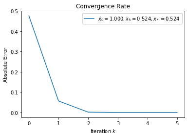
(a)

\[\begin{split}f(x) &= \sin{(x)} - \cos{(2 x)}\\ f'(x) &= \cos{(x)} - (-2 \sin{(2 x)}) = \cos{(x)} + 2 \sin{(2 x)}\end{split}\]

Newton’s method will converge \(q\)-quadratically given \(x_0 = 1\) because \(x_* \in [0, 1]\) and within that range, \(\exists \rho > 0\) such that \(\left| f'(x) \right| > \rho\).

hqn = HybridQuasiNewton()
f = lambda x: numpy.sin(x) - numpy.cos(2 * x)
x_0 = 1
x_star = 0.523598775598

solver = lambda x: hqn.evaluate_secant(f, x)
plot_convergent_sequence(solver, x_0, x_star)

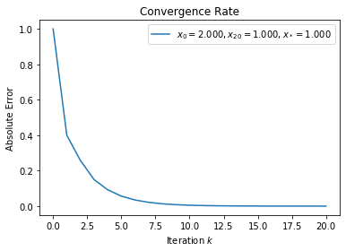
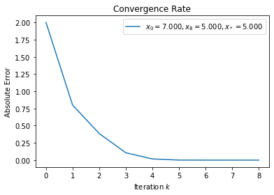
(b)

\[\begin{split}f(x) &= x^3 - 7 x^2 + 11 x - 5\\ f'(x) &= 3 x^2 - 14 x + 11\end{split}\]

Newton’s method will converge \(q\)-quadratically to \(x_* = 5\) when \(x_0 = 7\). When \(x_0 = 2\), it will converge \(q\)-linearly to \(x_* = 1\) because \(f'(x_* = 1) = 0\) i.e. the multiple roots at \(x_*\) violate the \(\rho > 0\) condition.

hqn = HybridQuasiNewton()
f = lambda x: x**3 - 7 * x**2 + 11 * x - 5
x_0 = 2
x_star = 1.00004066672

solver = lambda x: hqn.evaluate_secant(f, x)
plot_convergent_sequence(solver, x_0, x_star)

x_0 = 7
x_star = 5
plot_convergent_sequence(solver, x_0, x_star)

(c)

\[\begin{split}f(x) &= \sin{(x)} - \cos{(x)}\\ f'(x) &= \cos{(x)} + \sin{(x)}\end{split}\]

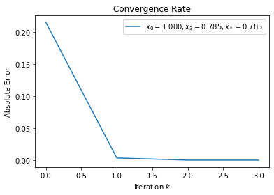
Newton’s method will converge \(q\)-quadratically when \(x_0 = 1\).

hqn = HybridQuasiNewton()
f = lambda x: numpy.sin(x) - numpy.cos(x)
x_0 = 1
x_star = 0.78539816335

solver = lambda x: hqn.evaluate_secant(f, x)
plot_convergent_sequence(solver, x_0, x_star)

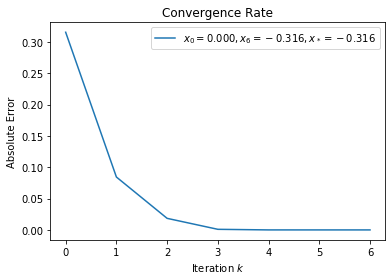
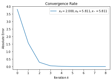
(d)

\[\begin{split}f(x) &= x^4 - 12 x^3 + 47 x^2 - 60 x - 24\\ f'(x) &= 4 x^3 - 36 x^2 + 94 x - 60\end{split}\]

Both \(x_0 = 0\) and \(x_0 = 2\) will achieve \(q\)-quadratic convergence with Newton’s method. However, \(x_0 = 2\)’s convergence is slower than \(x_0 = 0\)’s because there are two zero crossings for \(f'(x)\) on the way to \(x_*\).

hqn = HybridQuasiNewton()
f = lambda x: x**4 - 12 * x**3 + 47 * x**2 - 60 * x - 24
x_0 = 0
x_star = -0.315551843713

solver = lambda x: hqn.evaluate_secant(f, x)
plot_convergent_sequence(solver, x_0, x_star)

x_0 = 2
x_star = 5.81115950152
plot_convergent_sequence(solver, x_0, x_star)

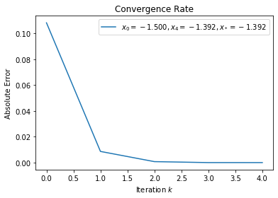
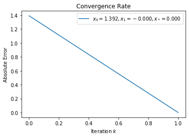
Exercise 10

\[\begin{split}x_+ &= x_c - \frac{\arctan{(x_c)}}{(1 + x_c^2)^{-1}}\\ &= x_c - \arctan{(x_c)}(1 + x_c^2)\end{split}\]

This formulation of Newton’s method will cycle when \(x_+ = -x_c\) such that

\[\begin{split}-x_c &= x_c - \arctan{(x_c)}(1 + x_c^2)\\ 0 &= 2 x_c - (1 + x_c^2) \arctan{(x_c)}.\end{split}\]

However, since Newton’s method was paired with backtracking, it will not cycle.

hqn = HybridQuasiNewton()
f = lambda x: 2 * x - (1 + x * x) * numpy.math.atan(x)
x_0 = -1.5
x_star = -1.39174520382

solver = lambda x: hqn.evaluate_secant(f, x)
plot_convergent_sequence(solver, x_0, x_star)

x_0 = 0.0001
x_star = 0
plot_convergent_sequence(solver, x_0, x_star)

x_0 = 1.5
x_star = 1.39174520382
plot_convergent_sequence(solver, x_0, x_star)

hqn = HybridQuasiNewton()
f = lambda x: numpy.math.atan(x)
x_0 = 1.39174520382
x_star = 0

solver = lambda x: hqn.evaluate_secant(f, x)
plot_convergent_sequence(solver, x_0, x_star)

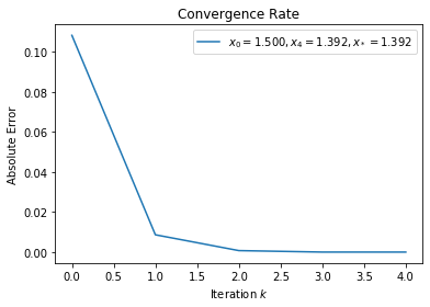
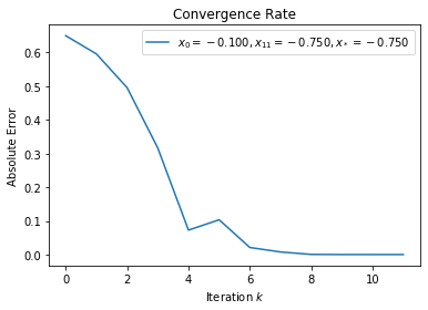
Exercise 11

To minimize a one variable \(f(x)\), a quadratic model of \(f(x)\) around \(x_c\) is created and the critical point of the model is subsequently solved for.

One such quadratic model is the second-order Taylor series

\[f(x) \approx f(x_c) + f'(x_c) (x - x_c) + \frac{1}{2}f''(x_c) (x - x_c)^2\]

such that

\[\begin{split}0 &= \frac{\partial f}{\partial x}\\ &= f'(x_c) + f''(x_c) (x - x_c)\\ x &= x_c - \frac{f'(x_c)}{f''(x_c)}.\end{split}\]

import numpy

class NewtonQuadraticSolver1D:
    def __init__(self, tau=None, typx=None):
        self._kEpsilon = numpy.finfo(float).eps
        self._kRootEpsilon = numpy.sqrt(self._kEpsilon)

        #parameters to solver
        self._tau = tau
        if tau is None:
            self._tau = (self._kRootEpsilon,) * 2

        self._typx = typx
        if typx is None:
            self._typx = (1,)

    def evaluate_newton(self, f, f_p1, f_p2, x_c):
        denom = f_p2(x_c)
        if denom > 0:
            x_k = x_c - f_p1(x_c) / denom
        else:
            x_k = x_c + f_p1(x_c) / denom

        x_n = self._backtracking_strategy(f, x_c, x_k)

        return self._stop(f, f_p1, x_c, x_n), x_n

    def _backtracking_strategy(self, f, x_c, x_n):
        while f(x_n) >= f(x_c):
            x_n = (x_c + x_n) / 2
        return x_n

    def _stop(self, f, f_prime, x_c, x_n):
        return abs(f_prime(x_n) * x_n / f(x_n)) < self._tau[0] or\
            abs(x_n - x_c) / max(abs(x_n), self._typx[0]) < self._tau[1]

nqs1d = NewtonQuadraticSolver1D()
f = lambda x: x**4 + x**3
f_p1 = lambda x: 4 * x**3 + 3 * x**2
f_p2 = lambda x: 12 * x**2 + 6 * x
x_star = -0.75
x_0 = -0.1

solver = lambda x: nqs1d.evaluate_newton(f, f_p1, f_p2, x)
plot_convergent_sequence(solver, x_0, x_star)

Exercise 12

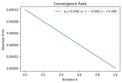
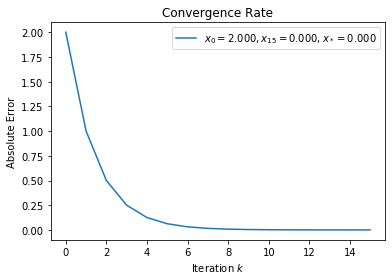
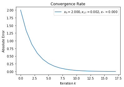
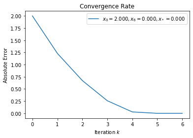
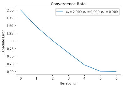
According to theorem 2.4.3, \(f(x) = x^2\) and \(f(x) = x^3\) converges q-linearly while \(f(x) = x + x^3\) and \(f(x) = x + x^4\) have q-quadratic convergence rate because \(f'(x_* = 0)\) must have a non-zero lower bound for Newton’s method to converge quadratically.

hqn = HybridQuasiNewton()
f = lambda x: x**2
f_p1 = lambda x: 2 * x
x_star = 0
x_0 = 2

solver = lambda x: hqn.evaluate_newton(f, f_p1, x)
plot_convergent_sequence(solver, x_0, x_star)

hqn = HybridQuasiNewton()
f = lambda x: x**3
f_p1 = lambda x: 3 * x**2
x_star = 0
x_0 = 2

solver = lambda x: hqn.evaluate_newton(f, f_p1, x)
plot_convergent_sequence(solver, x_0, x_star)

hqn = HybridQuasiNewton()
f = lambda x: x + x**3
f_prime = lambda x: 1 + 3 * x**2
x_star = 0
x_0 = 2

solver = lambda x: hqn.evaluate_newton(f, f_prime, x)
plot_convergent_sequence(solver, x_0, x_star)

hqn = HybridQuasiNewton()
f = lambda x: x + x**4
f_prime = lambda x: 1 + 4 * x**3
x_star = 0
x_0 = 2

solver = lambda x: hqn.evaluate_newton(f, f_prime, x)
plot_convergent_sequence(solver, x_0, x_star)

Exercise 13

Assume \(f(x)\) has \(n\) continuous derivatives on an interval about \(x = x_*\). \(f\) has a root (a.k.a. a zero) of multiplicity \(m\) at \(x_*\) if and only if

\[f(x_*) = f'(x_*) = \ldots = f^{(m - 1)}(x_*) = 0 \quad \text{and} \quad f^{(m)}(x_*) \neq 0.\]

The foregoing implies \(f\) can be factorized as

\[f(x) = \left( x - x_* \right)^m q(x)\]

where \(\lim_{x \to x_*} q(x) \neq 0\). Define \(e_{k + 1} = x_{k + 1} - x_*\) and \(e_k = x_k - x_*\). Newton’s method converges \(q\)-linearly to \(x_*\) because

\[\begin{split}x_{k + 1} - x_* &= x_k - x_* - \frac{f(x_k)}{f'(x_k)}\\ &= x_k - x_* - \frac{(x_k - x_*)^m q(x_k)}{ m (x_k - x_*)^{m - 1} q(x_k) + (x_k - x_*)^m q'(x_k) }\\ &= x_k - x_* - \frac{(x_k - x_*) q(x_k)}{m q(x_k) + (x_k - x_*) q'(x_k)}\\ \frac{x_{k + 1} - x_*}{x_k - x_*} &= 1 - \frac{q(x_k)}{m q(x_k) + (x_k - x_*) q'(x_k)}\\ &= \frac{m q(x_k) + (x_k - x_*) q'(x_k) - q(x_k)}{m q(x_k) + (x_k - x_*) q'(x_k)}\\ &= \frac{ m - 1 + (x_k - x_*) \frac{q'(x_k)}{q(x_k)} }{ m + (x_k - x_*) \frac{q'(x_k)}{q(x_k)} }\\ \lim_{k \to \infty} \frac{e_{k + 1}}{e_k} &= \frac{m - 1}{m}.\end{split}\]

Exercise 14

Assume \(f\) has \(n + 1\) continuous derivatives on an interval about \(x = x_*\) and satisfies

\[\begin{split}f'(x_*) &\neq 0,\\ f(x_*) &= f''(x_*) = \ldots = f^{(n)}(x_*) = 0,\\ f^{(n + 1)}(x_*) &\neq 0.\end{split}\]

By inspection, \(f\) can be factorized as

\[f(x) = (x - x_*)^{(n + 1)} q(x) + a (x - x_*)\]

where \(a \in \mathbb{R} \setminus \left\{ (x - x_*) \right\}\) and \(\lim_{x \to x_*} q(x) \neq 0\). Newton’s method converges \(q\)-cubicly to \(x_*\) because

\[\begin{split}x_{k + 1} - x_* &= x_k - x_* - \frac{f(x_k)}{f'(x_k)}\\ &= x_k - x_* - \frac{ (x_k - x_*)^{(n + 1)} q(x_k) + a (x_k - x_*) }{ (n + 1) (x_k - x_*)^{(n)} q(x_k) + (x_k - x_*)^{(n + 1)} q'(x_k) + a }\\ &= \frac{ (n + 1) (x_k - x_*)^{(n + 1)} q(x_k) + (x_k - x_*)^{(n + 2)} q'(x_k) + a (x_k - x_*) - (x_k - x_*)^{(n + 1)} q(x_k) - a (x_k - x_*) }{ (n + 1) (x_k - x_*)^{(n)} q(x_k) + (x_k - x_*)^{(n + 1)} q'(x_k) + a }\\ &= \frac{ n (x_k - x_*)^{(n + 1)} q(x_k) + (x_k - x_*)^{(n + 2)} q'(x_k) }{ (n + 1) (x_k - x_*)^{(n)} q(x_k) + (x_k - x_*)^{(n + 1)} q'(x_k) + a }\\ &= \frac{ n (x_k - x_*)^{(n + 1)} + (x_k - x_*)^{(n + 2)} \frac{q'(x_k)}{q(x_k)} }{ (n + 1) (x_k - x_*)^{(n)} + (x_k - x_*)^{(n + 1)} \frac{q'(x_k)}{q(x_k)} + \frac{a}{q(x_k)} }\\ \left| x_{k + 1} - x_* \right| &= \left\vert \frac{ n (x_k - x_*)^{(n + 1)} + (x_k - x_*)^{(n + 2)} \frac{q'(x_k)}{q(x_k)} }{ (n + 1) (x_k - x_*)^{(n)} + (x_k - x_*)^{(n + 1)} \frac{q'(x_k)}{q(x_k)} + \frac{a}{q(x_k)} } \right\vert\\ &= \frac{1}{\rho} \left\vert n (x_k - x_*)^{(n + 1)} + (x_k - x_*)^{(n + 2)} \frac{q'(x_k)}{q(x_k)} \right\vert\\ &\leq \frac{\gamma}{\rho} \left\vert x_k - x_* \right\vert^{(n + 1)}\end{split}\]

where \(\rho, \gamma > 0\).

Exercise 15

\[\begin{split}0 &\approx M(x)\\ &= f(x_c) + f'(x_c) (x - x_c) + \frac{1}{2} f''(x_c) (x - x_c)^2\\ &= \frac{f(x_c)}{f''(x_c)} + \frac{f'(x_c)}{f''(x_c)} (x - x_c) + \frac{1}{2} (x - x_c)^2\\ &= \frac{f(x_c)}{f''(x_c)} + \frac{f'(x_c)}{f''(x_c)} x - \frac{f'(x_c)}{f''(x_c)} x_c + \frac{1}{2} x^2 - x x_c + \frac{1}{2} x_c^2\\ &= \frac{1}{2} x^2 + \left( \frac{f'(x_c)}{f''(x_c)} - x_c \right) x + \frac{1}{2} x_c^2 - \frac{f'(x_c)}{f''(x_c)} x_c + \frac{f(x_c)}{f''(x_c)}\\ &= a x^2 + b x + c\end{split}\]

An exact solution to the foregoing quadratic equation is

\[\begin{split} x &= \frac{-b \pm \sqrt{b^2 - 4 a c}}{2 a}\\ &= -\left(\frac{f'(x_c)}{f''(x_c)} - x_c \right) \pm \sqrt{\left(\frac{f'(x_c)}{f''(x_c)} - x_c \right)^2 - 2 c}\\ &= x_c - \frac{f'(x_c)}{f''(x_c)} \pm \sqrt{ \left(\frac{f'(x_c)}{f''(x_c)} \right)^2 - 2 \frac{f'(x_c)}{f''(x_c)} x_c + x_c^2 - x_c^2 + 2 \frac{f'(x_c)}{f''(x_c)} x_c - 2 \frac{f(x_c)}{f''(x_c)} }\\ &= x_c - \frac{f'(x_c)}{f''(x_c)} \pm \sqrt{ \left( \frac{f'(x_c)}{f''(x_c)} \right)^2 - 2 \frac{f(x_c)}{f''(x_c)} }\\ &= x_c - \frac{f'(x_c) \pm \sqrt{f'(x_c)^2 - 2 f(x_c) f''(x_c)}}{f''(x_c)}.\end{split}\]

There are two (possibly three) major issues with this approach. The first is loss of significance due to the square root operation. The second is when \(f'(x_c)^2 \gg 2 f(x_c) f''(x_c)\) or \(f'(x_c)^2 \sim 2 f(x_c) f''(x_c)\). Lastly, \(x_k\) can be complex even if all the previous iterates were real.

A quadratic model is appropriate when the affine model is not satisfactory with respect to the desired criteria. It turns out this is equivalent to Halley’s irrational method [Ack].

Exercise 16

Assume \(f \in C^1(D)\), \(x_c \in D\), \(f(x_c) \neq 0\), \(f'(x_c) \neq 0\), and \(\mathrm{d} = -f(x_c) / f'(x_c)\).

\[\begin{split}f(x_c + \lambda \mathrm{d}) - f(x_c) &= \int_0^\lambda \mathrm{d} f'(x_c + \alpha \mathrm{d}) d\alpha\\ &= \int_0^\lambda \frac{-f(x_c)}{f'(x_c)} f'(x_c + \alpha \mathrm{d}) d\alpha\\ 1 - \frac{f(x_c + \lambda \mathrm{d})}{f(x_c)} &= \int_0^\lambda \frac{f'(x_c + \alpha \mathrm{d})}{f'(x_c)} d\alpha\\ &> 0.\end{split}\]

Choose \(t\) such that \(f'(x_c + \lambda d) f'(x_c) > 0\) for all \(\lambda \in (0, t)\).

\[\begin{split}1 &> \frac{f(x_c + \lambda \mathrm{d})}{f(x_c)}\\ \frac{ \left\vert f(x_c) \right\vert }{ \left\vert f(x_c + \lambda \mathrm{d}) \right\vert } &> \frac{ \text{sgn}\left( f(x_c + \lambda \mathrm{d}) \right) }{ \text{sgn}\left( f(x_c) \right) }\\ \left\vert f(x_c) \right\vert &> \left\vert f(x_c + \lambda \mathrm{d}) \right\vert \text{sgn}\left( f(x_c + \lambda \mathrm{d}) f(x_c) \right).\end{split}\]

This illustrates that once the minimizing point \(x_*\) is almost reached using the suggested \(\mathrm{d}\) step size, the optimization can stop. However, this only works when the region has the same sign.

Exercise 17

\[\frac{ \left| x_+ - x_c \right| }{ \max \left\{ \left| x_+ \right|, \left| x_c \right| \right\} } < 10^{-7}\]

will not be satisfied for \(f(x) = x^2\) because the relative error is constant (either 0.5 or 1.0) at each time step.

\[\frac{ \left| x_+ - x_c \right| }{ \max \left\{ \left| x_+ \right|, \text{typ}x \right\} } < 10^{-7}\]

will be satisfied with an appropriately selected \(\text{typ}x\).

f = lambda x: x**2
f_prime = lambda x: 2 * x
x_star = 0
x_c = 1

METHODS = ['Absolute Error',
           'Current Value',
           'Relative Error',
           'Satisfy Condition']
STR_FMT = '{0!s:16}\t{1!s:16}\t{2!s:16}\t{3!s:16}'
print(STR_FMT.format(*METHODS))

typx = 1
SC = []
X_i = [x_c]
for i in range(0, 20):
    x_k = Newtons_Method(f, f_prime, x_c)
    x_c = x_k

    X_i.append(x_k)
    top = abs(X_i[i + 1] - X_i[i])
    bot = max(abs(X_i[i + 1]), abs(typx))
    print(STR_FMT.format(abs(x_k - x_star), f(x_k), top / bot,
                         (f(x_k) < 10e-5, top / bot < 10e-7)))

Absolute Error          Current Value           Relative Error          Satisfy Condition
0.5                     0.25                    0.5                     (False, False)
0.25                    0.0625                  0.25                    (False, False)
0.125                   0.015625                0.125                   (False, False)
0.0625                  0.00390625              0.0625                  (False, False)
0.03125                 0.0009765625            0.03125                 (False, False)
0.015625                0.000244140625          0.015625                (False, False)
0.0078125               6.103515625e-05         0.0078125               (True, False)
0.00390625              1.52587890625e-05       0.00390625              (True, False)
0.001953125             3.814697265625e-06      0.001953125             (True, False)
0.0009765625            9.5367431640625e-07     0.0009765625            (True, False)
0.00048828125           2.384185791015625e-07   0.00048828125           (True, False)
0.000244140625          5.960464477539063e-08   0.000244140625          (True, False)
0.0001220703125         1.4901161193847656e-08  0.0001220703125         (True, False)
6.103515625e-05         3.725290298461914e-09   6.103515625e-05         (True, False)
3.0517578125e-05        9.313225746154785e-10   3.0517578125e-05        (True, False)
1.52587890625e-05       2.3283064365386963e-10  1.52587890625e-05       (True, False)
7.62939453125e-06       5.820766091346741e-11   7.62939453125e-06       (True, False)
3.814697265625e-06      1.4551915228366852e-11  3.814697265625e-06      (True, False)
1.9073486328125e-06     3.637978807091713e-12   1.9073486328125e-06     (True, False)
9.5367431640625e-07     9.094947017729282e-13   9.5367431640625e-07     (True, True)

Exercise 18

Choose \(\widehat{D} \subset D\) such that \(\left| f'(x) \right| \leq \alpha\) for all \(x \in \widehat{D}\) where \(\alpha > 0\).

\[\begin{split}f(x) - f(x_*) &= \int_{x_*}^x f'(z) dz\\ \left\vert f(x) \right\vert &= \left\vert \int_{x_*}^x f'(z) dz \right\vert\\ &\leq \left\vert \int_{x_*}^x \alpha dz \right\vert\\ &= \alpha \left\vert \left. z \right|_{x_*}^x \right\vert\\ &= \alpha \left\vert x - x_* \right\vert.\end{split}\]

Exercise 19

The following is one way of deriving the forward finite difference formula for first order derivative of \(f\) using Taylor expansion at \(x\):

\[\begin{split}f(x + h) &\approx f(x) + h f'(x)\\ f'(x) &\approx \frac{f(x + h) - f(x)}{h}.\end{split}\]

Invoking Corollary 2.6.2 and the derivations in Exercise 20 gives

\[\begin{split}\left| \frac{f(x_c + h_c) - f(x_c)}{h_c} - f'(x_c) \right| &\leq \left| \frac{ f(x_c + h_c) + \eta |f(x_c + h_c)| - f(x_c) - \eta |f(x_c)| }{h_c} - f'(x_c) \right|\\ &\leq \left| \frac{ f(x_c + h_c) - f(x_c)}{h_c} - f'(x_c) + \eta \frac{|f(x_c + h_c)| - |f(x_c)| }{h_c} \right|\\ &\leq \left| \frac{f(x_c + h_c) - f(x_c)}{h_c} - f'(x_c) \right| + \left| \eta \frac{|f(x_c + h_c)| + |f(x_c)|}{h_c} \right|\\ &\leq \frac{\gamma \left| h_c \right|}{2} + \eta \frac{|f(x_c + h_c)| + |f(x_c)|}{|h_c|}.\end{split}\]

Assuming \(f(x_c + h_c) \cong f(x_c)\),

\[\begin{split}0 &\leq \frac{\gamma \left| h_c \right|}{2} + \eta \frac{|f(x_c + h_c)| + |f(x_c)|}{|h_c|}\\ 0 &\cong \frac{\gamma}{2} h_c^2 + 2 \eta |f(x_c)|\\ h_c &\approx \pm \sqrt{\frac{- 4 \eta |f(x_c)|}{\gamma}}\\ &\approx \pm 2i \sqrt{\frac{\eta |f(x_c)|}{\gamma}}.\end{split}\]

Note that if \(|f'(x)| \ll |f(x)|\), then the finite difference is going to evaluate to zero before ever reaching \(f'(x)\)’s vicinity because \(\text{fl}(f(x + h)) = \text{fl}(f(x))\).

Exercise 20

A couple useful facts to recall are

• \(f'' \in \text{Lip}_\gamma(D)\) implies \(f''\) is continuously differentiable, which means \(f'''\) exists and is itself a continous function.

• Any function can be written as \(f(z) \approx T_n(z) + R_n(z)\) where \(T_n(z)\) is the \(n\)-th degree Taylor polynomial of \(f\) at \(x\) and

  \[R_n(z) = \frac{1}{n!} \int_x^z (z - t)^n f^{(n + 1)}(t) dt\]

  is the remainder of the series.

• Weighted Mean Value Theorem for Integrals.

  • If \(f\) and \(g\) are continuous on \([a, b]\) and \(g\) does not change sign in \([a, b]\), then there exists \(c \in [a, b]\) such that

    \[\int_a^b f(x) g(x) dx = f(c) \int_a^b g(x) dx.\]

Observe that when \(n = 2\) and \((z - t)^n\) does not change sign in the interval \([x, z]\),

\[\begin{split}\left| f(z) - T_n \right| &\leq \left| R_n(z) \right|\\ &= \left| \frac{1}{n!} \int_x^z (z - t)^n f^{(n + 1)}(t) dt \right|\\ &= \frac{\gamma}{n!} \left| \int_x^z (z - t)^n dt \right|\\ &= \frac{\gamma}{n!} \left| \left. -\frac{(z - t)^{n + 1}}{n + 1} \right|_x^z \right|\\ &= \frac{\gamma}{(n + 1)!} \left| z - x \right|^{n + 1}\\ &= \frac{\gamma}{6} \left| z - x \right|^{3}.\end{split}\]

A more rigorous proof would involve the Squeeze Theorem bounding \(R_n(z)\) as \(x \to z\) from the left and right side.

The following is one way of deriving the central difference formula for second order derivative of \(f\) using Taylor expansion at \(x\):

\[\begin{split}f(x + h) &\approx f(x) + h f'(x) + \frac{h^2}{2}f''(x)\\ f(x - h) &\approx f(x) - h f'(x) + \frac{h^2}{2}f''(x)\\ f(x + h) + f(x - h) &\approx 2 f(x) + h^2 f''(x)\\ f''(x) &\approx \frac{f(x + h) - 2 f(x) + f(x - h)}{h^2}.\end{split}\]

The following illustrates that the central difference formula has a tighter upper bound via invoking the previous derivations with \(z = x_c + h_c\) and \(x = x_c\).

\[\begin{split}\left| f(x_c + h_c) - f(x_c) - h_c f'(x_c) - \frac{h_c^2}{2} f''(x_c) \right| &\leq \frac{\gamma}{6} \left| h_c \right|^3\\ \left| f(x_c + h_c) - f(x_c) - h_c f'(x_c) - \frac{h_c^2}{2} \left( \frac{f(x_c + h_c) - 2 f(x_c) + f(x_c - h_c)}{h_c^2} \right) \right| &\leq \frac{\gamma}{6} \left| h_c \right|^3\\ \left| f(x_c + h_c) - f(x_c) - h_c f'(x_c) - \frac{1}{2} f(x_c + h_c) + f(x_c) - \frac{1}{2} f(x_c - h_c) \right| &\leq \frac{\gamma}{6} \left| h_c \right|^3\\ \left| \frac{f(x_c + h_c) - f(x_c - h_c)}{2} - h_c f'(x_c) \right| &\leq \frac{\gamma}{6} \left| h_c \right|^3\\ \left| \frac{f(x_c + h_c) - f(x_c - h_c)}{2 h_c} - f'(x_c) \right| &\leq \frac{\gamma}{6} \left| h_c \right|^2\\ \left| a_c - f'(x_c) \right| &\leq \frac{\gamma}{6} \left| h_c \right|^2.\end{split}\]

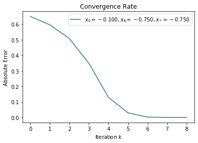
Exercise 21

As demonstrated in Exercise 9, one approach is to compute the central finite difference for \(f''(x)\) using \(f'(x)\) and then apply the secant approximation to the forward finite difference for subsequent iterations.

import numpy

class SecantQuadraticSolver1D:
    def __init__(self, tau=None, typx=None):
        self._kEpsilon = numpy.finfo(float).eps
        self._kRootEpsilon = numpy.sqrt(self._kEpsilon)

        #parameters to solver
        self._tau = tau
        if tau is None:
            self._tau = (self._kRootEpsilon,) * 2

        self._typx = typx
        if typx is None:
            self._typx = (1,)

        self._secant_state = None

    def evaluate_cfd(self, f, f_p1, x_c):
        h_c = self._kRootEpsilon * max(abs(x_c), self._typx[0])
        denom = (f_p1(x_c + h_c) - f_p1(x_c - h_c)) / (2 * h_c)
        if denom > 0:
            x_k = x_c - f_p1(x_c) / denom
        else:
            x_k = x_c + f_p1(x_c) / denom

        x_n = self._backtracking_strategy(f, x_c, x_k)

        return self._stop(f, f_p1, x_c, x_n), x_n

    def evaluate(self, f, fp, x_c):
        if self._secant_state is None:
            #first iteration, so no previous results to use
            h_c = self._kRootEpsilon * max(abs(x_c), self._typx[0])
            #compute central finite difference
            a_c = (fp(x_c + h_c) - fp(x_c - h_c)) / (2 * h_c)

            #evaluate local model
            fp_xc = fp(x_c)
            if a_c > 0:
                x_k = x_c - fp_xc / a_c
            else:
                x_k = x_c + fp_xc / a_c

            self._secant_state = (x_c, fp_xc)
        else:
            #define h_c = x_previous - x_current
            x_, fp_x_ = self._secant_state

            #evaluate model with secant approximation
            fp_xc = fp(x_c)
            a_c = (fp_x_ - fp_xc) / (x_ - x_c)
            if a_c > 0:
                x_k = x_c - fp_xc / a_c
            else:
                x_k = x_c + fp_xc / a_c

            self._secant_state = (x_c, fp_xc)

        x_n = self._backtracking_strategy(f, x_c, x_k)

        return self._stop(f, fp, x_c, x_n), x_k

    def _backtracking_strategy(self, f, x_c, x_n):
        f_xc = f(x_c)
        while f(x_n) >= f_xc:
            x_n = (x_c + x_n) / 2
        return x_n

    def _stop(self, f, f_prime, x_c, x_n):
        return abs(f_prime(x_n) * x_n / f(x_n)) < self._tau[0] or\
            abs(x_n - x_c) / max(abs(x_n), self._typx[0]) < self._tau[1]

f = lambda x: x**4 + x**3
f_p1 = lambda x: 4 * x**3 + 3 * x**2
x_star = -0.75
x_0 = -0.1

sqs1d = SecantQuadraticSolver1D()
solver = lambda x: sqs1d.evaluate(f, f_p1, x)
plot_convergent_sequence(solver, x_0, x_star)

References

Ack

Peter John Acklam. A small paper on halley’s method. http://web.archive.org/web/20151030212505/http://home.online.no/ pjacklam/notes/halley/halley.pdf. Accessed on 2017-01-28.

Gay79

David M Gay. Some convergence properties of broyden’s method. SIAM Journal on Numerical Analysis, 16(4):623–630, 1979.

Pot89

FA Potra. On q-order and r-order of convergence. Journal of Optimization Theory and Applications, 63(3):415–431, 1989.